Using Wolfram Mathematica to Optimise Inventory Management

Introduction

The optimisation of inventory levels represents a fundamental challenge in contemporary business operations, characterised by the delicate balance between excess stock and potential stock-outs. This critical trade-off manifests in substantial holding costs on one end of the spectrum and lost revenue opportunities on the other, making the determination of optimal stock levels an essential aspect of operational efficiency.

This article presents a practical approach to inventory optimisation through the application of Wolfram Engine, a free version of the powerful Wolfram Mathematica platform. Unlike traditional approaches that often rely on heuristics, we demonstrate how mathematical modelling can transform inventory management into a precise, data-driven discipline. Our methodology harnesses the computational capabilities of the Wolfram Engine to solve complex inventory optimisation problems whilst maintaining accessibility for real-world implementation.

The following analysis offers a comprehensive examination of inventory optimisation techniques, suitable for both operations research specialists and practitioners new to mathematical optimisation. Through systematic exploration of key concepts and step-by-step implementation, we demonstrate how the Wolfram Engine's analytical framework can be effectively utilised to achieve optimal inventory management solutions. Importantly, we focus on practical applications that can be implemented using the free Wolfram Engine, making these sophisticated optimisation techniques accessible to organisations of all sizes.

Understanding the Problem

Let's consider Barista's Best, a specialty coffee roastery in Melbourne that supplies their premium Ethiopian Yirgacheffe beans to local cafés. Here's their inventory management challenge:

1. Daily Demand: On average, they sell 50 one-kilogram bags of these specialty beans daily to cafés across the city. However, demand fluctuates significantly - sometimes dropping to 30 bags during quiet periods or spiking to 70 bags when several cafés run promotions or during major events like the Melbourne Food & Wine Festival.

2. Holding Costs: Each kilogram of coffee beans costs $1.20 per day to store properly. This includes climate-controlled storage to maintain freshness $0.70, insurance $0.30, and handling costs $0.20. Green coffee beans also gradually lose quality over time, adding to the urgency of optimal stock management.

3. Stockout Costs: When Barista's Best can't fulfil a café's order, they face multiple penalties:

• lost immediate sale $15 profit per kg,

• risk of damaging long-term café relationships $50 estimated future value per incident,

• emergency shipping from their Sydney warehouse $200 per shipment,

• potential loss of café customers to competitors who might offer more reliable supply.

4. Goal: Determine the optimal reorder point for their Ethiopian Yirgacheffe beans that minimises total costs while maintaining their reputation for reliable supply. The solution must account for the 3-day lead time from their importers and the beans' 6-month shelf life.

This real-world scenario demonstrates how complex inventory management becomes when dealing with perishable, premium products in a competitive market with demanding business customers.

Why Use Wolfram Mathematica?

Wolfram Mathematica is a software tool designed for solving mathematical problems, running simulations, and visualising data. Its flexibility allows us to:

• Simulate real-world scenarios (like varying daily demand).

• Calculate and compare costs for different reorder points.

• Find the stock level that minimises total costs.

Even if you’ve never used Mathematica, don’t worry—this guide is designed to be beginner-friendly.

Step-by-Step Walkthrough

Here’s how we’ll solve the problem described above using Mathematica:

Step 1: Define the Problem Parameters

We will account for:

• Daily Demand: Normally distributed with a mean of 50 bags and a standard deviation that accounts for variability (e.g., ±10 units).

• Holding Costs: $1.20 per kilogram per day (including storage, insurance, handling, and freshness loss).

• Stockout Costs:

  • $15 for lost immediate sale per unit,

  • $50 for potential long-term café relationship damage per incident,

  • $200 emergency shipping cost per stockout event.

• Reorder Points: Test stock levels ranging from 30 to 70 bags.

• Lead Time: 3 days from importers.

• Shelf Life: 180 days (6 months).

In Mathematica, this looks like:

(* Parameters *)

meanDemand = 50; (* Average daily demand (in kg) *)

stdDevDemand = 10; (* Standard deviation of daily demand *)

holdingCostPerUnit = 1.2; (* Daily holding cost per kg *)

(* Stockout costs *)

immediateLossPerUnit = 15; (* Lost profit per unit *)

relationshipLossPerIncident = 50; (* Estimated future value loss per incident *)

emergencyShippingCost = 200; (* Emergency shipping cost per shipment *)

leadTime = 3; (* Lead time in days *)

shelfLife = 180; (* Shelf life in days *)

(* Reorder points: test levels between 30 and 70 kg *)

reorderPoints = Range[30, 70, 1]; (* Potential reorder points *)

Step 2: Simulate Daily Demand

We’ll use a normal distribution to simulate daily demand. A normal distribution models data where most values are near the average (50 kg in this case), but some can vary above or below.

In Mathematica:

(* Simulate 1,000 days of daily demand using a normal distribution *)

dailyDemand = RandomVariate[NormalDistribution[meanDemand, stdDevDemand], 1000];

(* Constrain demand to be non-negative *)

dailyDemand = Select[dailyDemand, # >= 0 &];

Normal Distribution:

• Simulates daily demand based on the given mean (meanDemand = 50) and standard deviation (stdDevDemand = 10).

• This reflects real-world variability where demand is centered around the mean but fluctuates.

Non-Negative Constraint:

• Ensures that demand values are non-negative (Select[dailyDemand, # >= 0 &]), as it’s not realistic to have negative demand.

1,000 Days of Simulation:

• The simulation generates 1,000 daily demand values to represent a realistic sample of café demand over time.

You can visualise the simulated demand distribution to ensure it aligns with expectations:

(* Visualise the simulated demand distribution *)

Histogram[dailyDemand, 20, "Probability", PlotLabel -> "Simulated Daily Demand Distribution"]

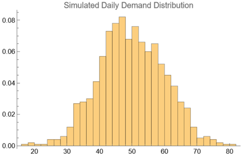
As expected, the histogram shows a bell curve centred around 50, with values mostly within the range of 30 - 70, consistent with the scenario described above.

Step 3: Calculate Costs and the Optimal Reorder Point

For each reorder point, we have the following parameters:

Holding Costs: $1.20 per kg per day for any excess stock.

Stockout Costs:

• $15 per kg for lost sales.

• $50 per incident for relationship damage.

• $200 for emergency shipping if stockout occurs.

In Mathematica, we can combine these into the following calculations:

(* Find optimal reorder point *)

optimalReorderPoint = reorderPoints[[FirstPosition[costs, Min[costs]][[1]]]];

ListLinePlot[

Transpose[{reorderPoints, costs}],

Frame -> True,

FrameLabel -> {"Reorder Point (kg)", "Total Cost ($)"},

PlotStyle -> {Thick, Aqua},

PlotMarkers -> Automatic,

PlotLabel -> "Costs vs. Reorder Points",

ImageSize -> Large,

(*PlotRangePadding -> {Scaled[0.1], Scaled[0.4]}, (* Add more vertical padding for text clearance *)*)

Epilog -> {

Green,

PointSize[Medium],

Point[{optimalReorderPoint, Min[costs]}],

Text[

Style[

StringJoin[

"{",ToString[optimalReorderPoint],

"; $", ToString[Round[Min[costs], 0.1]],"}"

],

Black, 6 (* Adjust font size for visibility *)

],

{optimalReorderPoint, Min[costs]},

{0.5, 2.25} (* Center alignment for the text *)

]

}

]

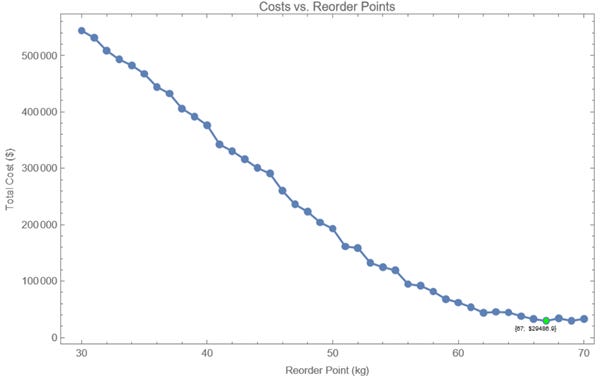
Results

Optimal Reorder Point: Mathematica calculates the reorder point (e.g., 67 kg) that minimises costs.

Cost Visualisation: The plot shows how costs change with stock levels, reaching the value of $29,480 at the optimal reorder point.

Practical Applications

You can adapt this approach to:

• Retail Stores: Optimise stock levels for perishable goods to avoid waste.

• Manufacturing: Balance production schedules and inventory to minimise downtime.

• E-commerce: Manage warehouse stock for high-demand items.

Benefits

This example demonstrates the power of tools like Mathematica in helping businesses, such as specialty coffee roasteries, make precise, data-driven decisions. By simulating real-world scenarios - such as fluctuating daily demand, holding costs, and the risks of stockouts - and applying mathematical optimisation, businesses can identify strategies that minimize costs while maintaining reliable supply chains.

In this case, Barista's Best can achieve significant benefits:

1. Cost Savings: Optimize inventory levels to reduce holding costs while avoiding expensive emergency shipments.

2. Improved Customer Relationships: Ensure consistent order fulfilment, strengthening long-term partnerships with café clients.

3. Waste Reduction: Manage perishable inventory like coffee beans more effectively, reducing spoilage and maximizing product quality.

4. Operational Efficiency: Streamline decision-making processes by relying on clear, data-backed insights rather than guesswork.

By leveraging Mathematica's capabilities for demand simulation, cost modelling, and visualization, businesses can confidently navigate complex inventory challenges, turning data into actionable insights that drive profitability and growth.

Conclusion

This case study demonstrates how Wolfram Mathematica can address a critical business challenge: optimising inventory to minimize costs while maintaining operational efficiency. By simulating real-world scenarios, accounting for fluctuations in demand, and modelling cost factors, we developed a robust and actionable framework that goes beyond trial-and-error decision-making.

The benefits of this approach extend far beyond the coffee roastery industry. Businesses in retail, manufacturing, logistics, healthcare, and even technology can leverage Mathematica’s capabilities to:

• Optimise Inventory Levels: Reduce holding costs and mitigate the risks of stockouts, whether managing raw materials, finished goods, or perishable items.

• Improve Resource Allocation: Dynamically adjust supply chains based on demand patterns, seasonal trends, or promotional activities.

• Enhance Customer Satisfaction: Minimize delays, prevent shortages, and ensure consistent delivery of goods or services.

• Drive Strategic Decision-Making: Use precise, data-driven insights to inform pricing strategies, warehouse operations, or distribution networks.

Mathematica’s versatility allows it to adapt to a variety of industries and challenges. From small businesses aiming to streamline operations to large enterprises optimizing complex supply chains, this framework offers a scalable solution that combines advanced mathematical modelling with practical, real-world applications.

By embracing tools like Mathematica, businesses not only save time but also gain a competitive edge, turning data into actionable insights that drive efficiency, cost savings, and growth. Whether you’re new to Mathematica or a seasoned operations professional, this methodology is a solid starting point for tackling inventory management and beyond.

Appendix: Getting Started with Wolfram Engive

The Wolfram Engine is freely available for developers and can be installed in a few simple steps:

1. Get Your Free License

- Visit https://www.wolfram.com/engine/

- Click "Get Engine for Developers"

- Create a Wolfram ID (free) if you don't have one

- Activate your free developer license

2. Installation

- Download the installer for your operating system (Windows, macOS, or Linux)

- Run the installer and follow the prompts

- When prompted, sign in with your Wolfram ID

- The installation process typically takes 5-10 minutes depending on your internet connection